Deep Dips #1: Multi-layer perceptrons

A new series exploring the components of deep learning

Deep learning is quite a thing these days, but it can be hard to find accessible yet factually correct guides to the bits and pieces that make it work. This new series is my attempt to fill this gap. It’s a deep dip, rather than a deep dive, since I’m going to focus on the big picture and explain the key ideas, rather than diving all the way down — though do check out the footnotes if you want to know more.

I’m going to start this series by talking about multilayer perceptrons (or MLP), which are fundamental components of most deep learning systems — or at least those based around neural networks¹. Neural networks are composed of artificial neurons. A perceptron is a kind of artificial neuron, and MLP is a neural network architecture created by stacking layers of perceptrons in a feedforward fashion. They were invented by Frank Rosenblatt way back in the middle of the last century², yet still play an important role in modern deep learning models such as transformers and convolutional neural networks (CNNs)³.

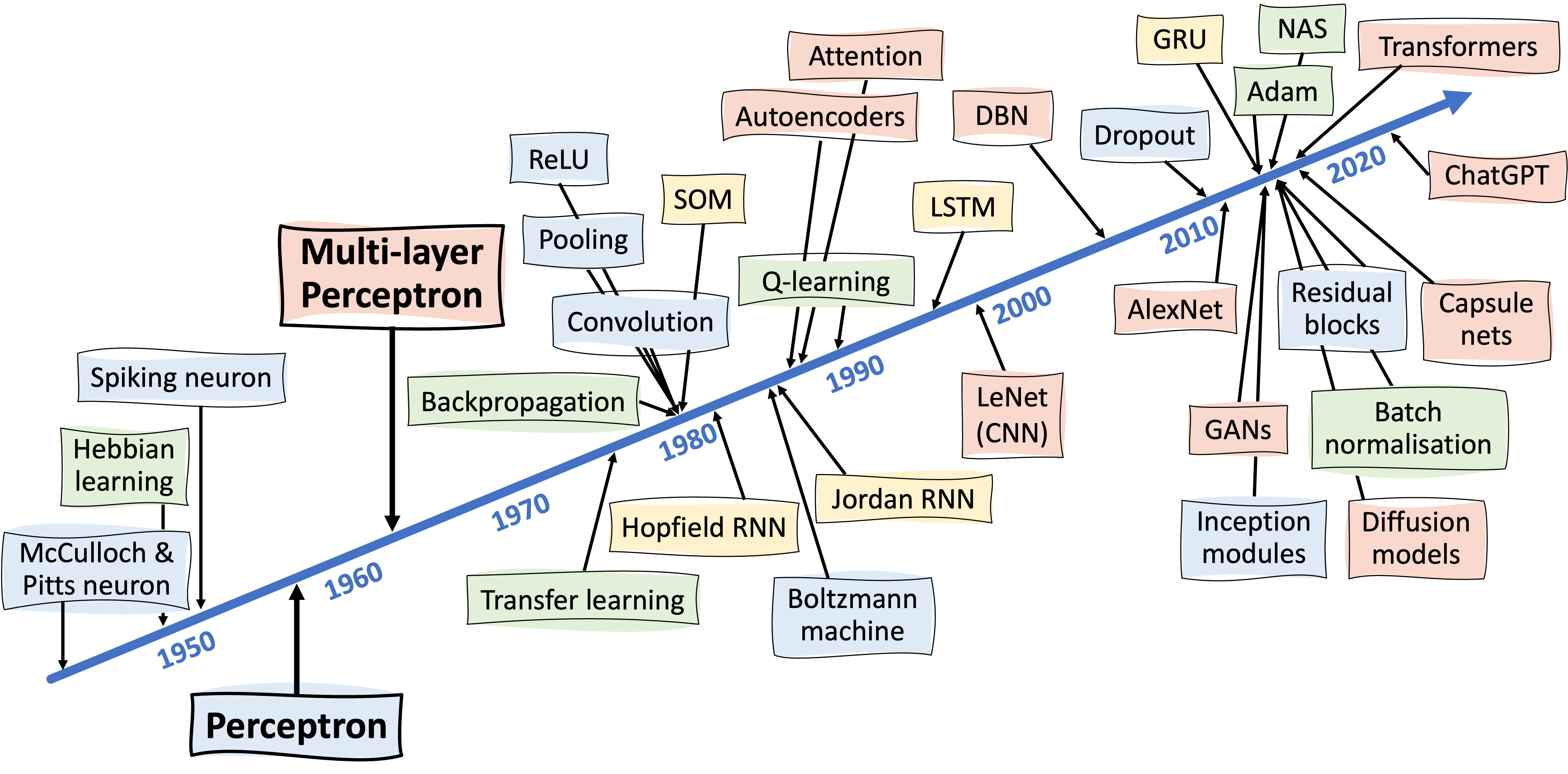
To put things in context, this timeline shows just how far back they appear in the history of deep learning — and indeed how far back many of the things we take for granted first appeared (also see Neural networks: everything changes but you):

I’ll begin with perceptrons, then move on to MLP, and finally I’ll say a bit about the universal approximation theory and what this tells us about the capabilities of MLP. There’s a TL;DR at the end for anyone with a limited attention span.

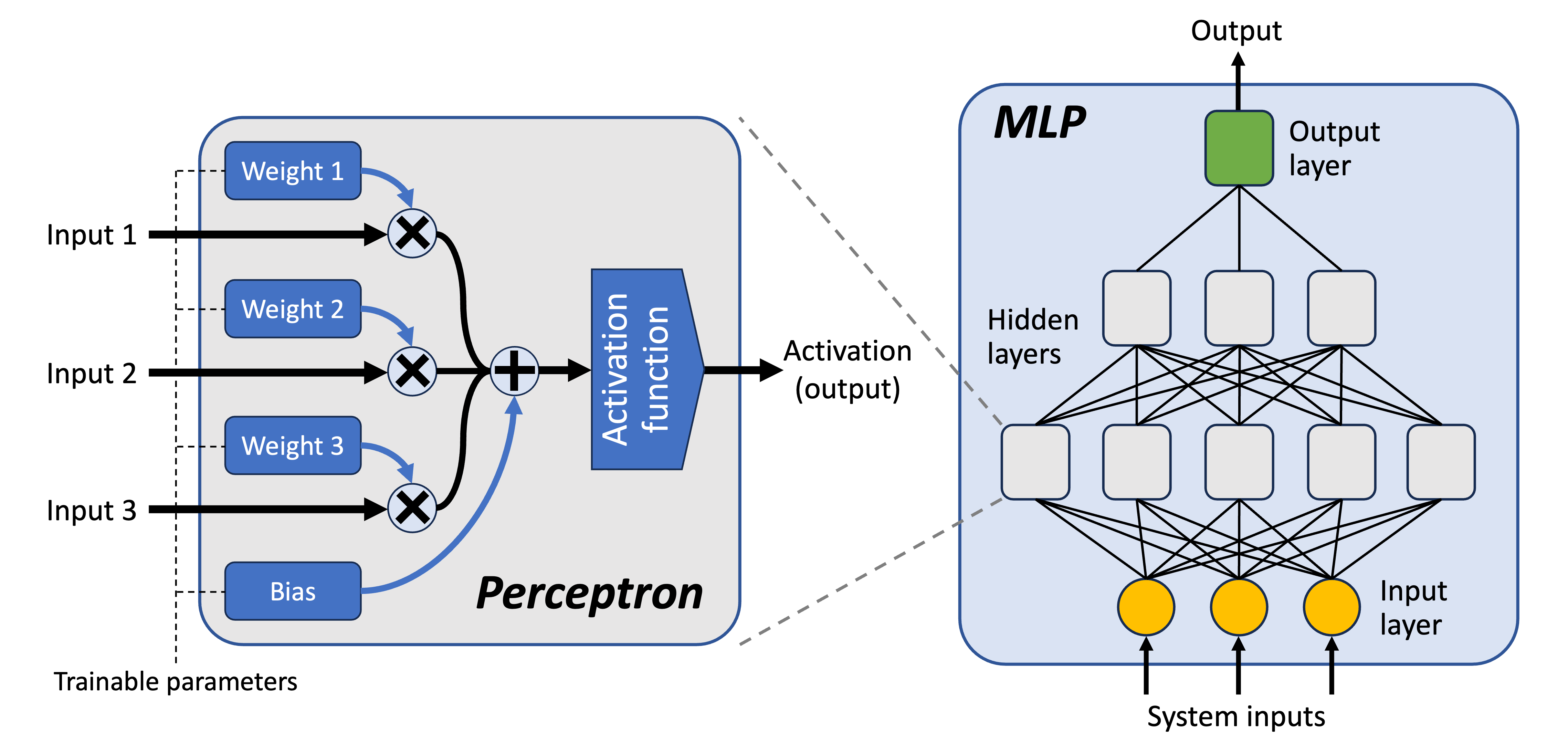
The following diagram shows how everything fits together, though note that things like the number of hidden layers and the number of inputs to a perceptron are configurable and will depend upon the problem being solved:

Perceptrons

A perceptron is a simple artificial neuron model that captures only the very basic behaviour of biological neurons.

Activation functions: At its heart is an activation function (also known as a transfer function), which is a mathematical function that takes one input and produces one output. This output then becomes the activation of the perceptron. When this is above a certain threshold, the neuron is said to be firing. Activation functions are usually monotonic, meaning that the output increases as the input increases, i.e. a larger input will always lead to a larger output. Most activation functions used these days are non-linear⁴, and this non-linearity is an important driver of complexity in neural networks. Most training algorithms also require activation functions to be differentiable⁵.

I’ll talk about specific activation functions in a future post, but most common are sigmoidal functions and rectified linear functions. Sigmoidal functions are often described as S-shaped, which basically means that until a certain input level, the output will be low. After this point, the output will grow rapidly — causing the perceptron to fire — until saturating at the function’s maximum output value. Rectified linear functions, by comparison, look like a bent stick; the first part is typically horizontal, and the second part points diagonally upwards. They tend to work better than sigmoidal functions as the number of layers in an MLP increases.

Weights: A perceptron receives multiple inputs. An important part of the process is how these multiple inputs are funnelled into the single input expected by its activation function. This is done by calculating a weighted sum. That is, each input has a weight (a number), and this weight is multiplied by the value received at the corresponding input (another number). These weighted inputs are then added together and become the input to the activation function. Weights can be positive or negative.

The process of training neural networks largely involves finding good values for these weights. Usually they start off with small random values⁶. Then, over the course of training, they’re gradually nudged towards more appropriate values — but more about training in a future post.

Biases: Perceptrons also have something called a bias. This is simply a value that’s added to the weighted sum of the inputs before it’s fed into the activation function. A bias acts as an offset, increasing or decreasing the input level required for a perceptron to fire. The bias is trained alongside the weights, and the weights and biases of the whole MLP are called its parameters.

Multilayer perceptrons

MLPs are formed by stacking layers of perceptrons in a feedforward manner. That is, the output activations of one layer of perceptrons typically⁷ become the inputs to the next layer. There are various ways of connecting them together, but a common approach is for all the outputs of one layer to become inputs to each perceptron in the next layer, i.e. each perceptron has a number of inputs equal to the number of perceptrons in the previous layer.

Input layer: The first layer, known as the input layer, is different. It’s just there to receive and transmit the MLP’s inputs⁸ further into the MLP. In fact, it doesn’t usually contain perceptrons; it just contains basic nodes that each receive one input and make it available to the perceptrons in the next layer. There are usually no weights, biases or activation functions.

Output layer: The final layer is known as the output layer. This contains one or more perceptrons, the number of which depend on the kind of problem that’s being solved. These perceptrons often use different activation functions to those in other layers. For instance, if the MLP is being used to solve a multi-class⁹ classification problem, there would typically be one perceptron in the output layer for each class, and these would use a softmax¹⁰ activation function. If it’s solving a regression problem, there’d usually be a single perceptron, and this would use a linear activation function¹¹.

Hidden layers: The layers in-between are known as the hidden layers, and this is where most of the business of the neural network gets done. One of the most important decisions when choosing an MLP architecture is the number of hidden layers to use, since this largely determines its capabilities. An MLP is usually considered to be “deep” when it has more than one or two hidden layers.

Once an MLP has been assembled and trained, it is executed in a synchronous manner, i.e. everything in a particular layer gets updated at the same time. The external inputs are first sucked into the input layer. The outputs of the input layer are then copied into the inputs of the first hidden layer. Once this is done, each of the perceptrons in this layer then do their thing, and their outputs are then copied to the inputs of the next layer. And so on, until the output layer gets some outputs. This process is often referred to as a forward pass, to distinguish it from the backward pass that is used in training¹².

Universal approximation theorem

The success of MLPs have a lot to do with the universal approximation theorem. This says that, given a few conditions, an MLP is capable of approximating any continuous function. This entails that they can capture pretty much any relationship between a group of inputs and a group of outputs, which makes MLPs a good basis for doing machine learning.

The conditions are pretty straightforward:

• First, there must be at least one hidden layer — check!

• Second, the activation functions must be non-linear — check!

• Third, there must be sufficient neurons in the hidden layer — erm…

So, how many neurons is sufficient? Well, the theorem says that an infinite number is definitely sufficient, but that’s not very useful guidance. Beyond that, no one really knows, and an important part of applying neural networks is determining whether you have enough neurons to solve the problem you’re applying it to. Usually this is a process of trial and error. A related question is how these neurons should be divided into hidden layers. The theorem doesn’t say you need more than one hidden layer, but in practice it’s hard to train a complex mapping if you don’t have more than one¹³.

And this raises another important limitation of the universal approximation theorem: it doesn’t say anything about training. Yes, it may say that a large enough MLP architecture with the right parameters can express a solution to the problem you’re trying to solve, but it doesn’t say whether a particular training algorithm can actually find the right parameters. But that’s a topic for another time.

Too Long, Didn’t Read

Despite being ancient, perceptrons and multilayer perceptrons (MLP) still play a big part in modern deep learning approaches. The nice thing about them is that they really are quite simple. A perceptron is just a non-linear function with weighted and summed inputs, and an MLP is just a bunch of perceptrons connected together in layers. In theory, we know they are capable of universal function approximation, which makes them a good bet for machine learning. However, getting the architecture right can be a fiddly process, and there’s no guarantee that a training algorithm will find the correct parameters.

1. Which is pretty much all of them, though the term deep learning is sometimes applied to deep versions of other machine learning models, such as decision trees and SVMs.

2. Building upon the earlier work of McCulloch and Pitts in the 1940s.

3. After applying convolution to extract features, a CNN normally feeds into an MLP to do the bulk of the decision making. In transformers, each block typically contains a self-attention layer followed by a couple of layers of MLP. More on this in future posts.

4. A lot of internet sources (including Wikipedia) state that perceptrons use linear activation functions. This is true of the first perceptron model, but it’s not true of later ones, including those used in Rosenblatt’s MLP.

5. -ish. Rectified linear functions aren’t differentiable at the bend.

6. There are various strategies for picking the initial values. This is somewhat tied to the choice of activation functions and optimiser, but typically you’d want the mean to be around zero, with most of the weights small to begin with, say between -0.2 and 0.2. Biases often start off at 0, but again this depends on activation functions and optimisers.

7. It is possible to have skip connections, where an output is routed to a layer beyond the next one. This is a big thing in modern deep learning models.

8. Which, in modern neural networks, will probably come from another part of the model, e.g. in a CNN, they’ll be the outputs of the convolution layers, and in a transformer they normally come after self-attention layers.

9. For a binary classification problem, only one output perceptron is required, usually with a sigmoidal activation function.

10. One softmax function is shared between the perceptrons of the output layer, and transforms the set of inputs that usually go to their individual activation functions (i.e. weighted sum + bias) into a set of pseudo-probability values, which then become the outputs.

11. Often the identity function, i.e. the output is just the weighted sum of inputs plus the bias.

12. At least for gradient-based optimisers.

13. It’s generally thought that MLPs build up progressively more complex representations of the input data over each subsequent layer. One other thing to bear in mind is that you do need at least one hidden layer: connecting the inputs directly to the output layer will only allow the MLP to solve linearly-separable problems.