Deep Dips #2: Embeddings and latent spaces

Last time in this series I talked about multilayer perceptrons, an old idea that still remains relevant to modern deep learning systems. This time I’m going to talk about another idea that has a been around a while, but which has recently become a key component of transformer models. These are embeddings, embedding spaces and latent spaces, which are all different terms for the same thing: a low-dimensional fixed-size representation of high-dimensional and often variable-length data. I’m going to start with autoencoders, which are the simplest kind of embedding, and then I’ll move onto word embeddings and also say a little about transformers (though these are covered in depth in the next post in this series, Deep Dips #3: Transformers).

Autoencoders

Like many great things in life, autoencoders are based on a simple yet effective idea: What happens when you train a neural network to output the same values that it receives at its inputs, whilst at the same time including a hidden layer that is narrower than its input and output layers? This narrow hidden layer is known as a bottleneck layer, and it forces the network to learn a compressed representation of its inputs.

The simplest autoencoders look something like this:

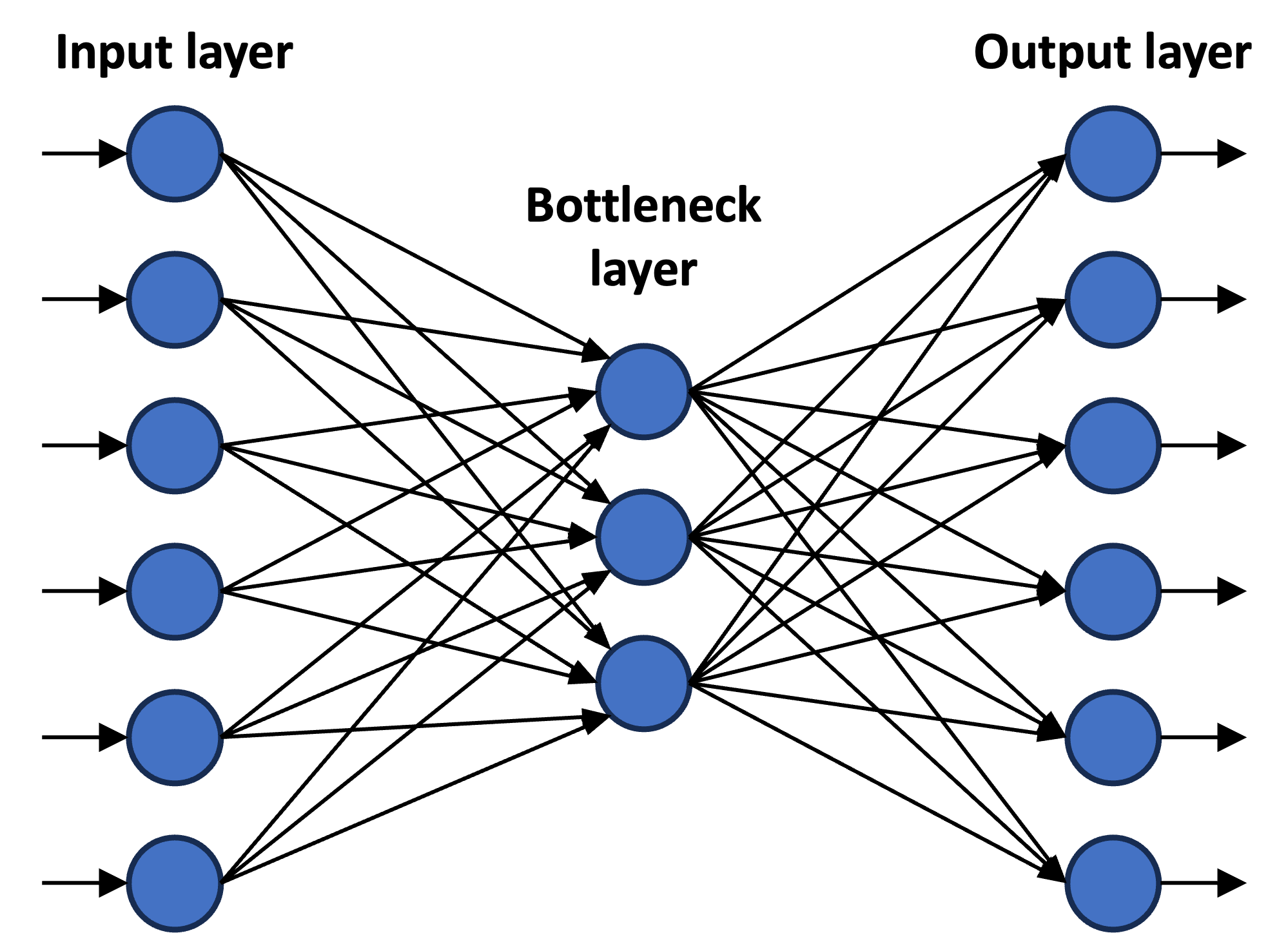
That is, they have one input layer where the data gets delivered, one output layer where the reconstructed data gets produced, and a single bottleneck layer. Using a standard neural network training algorithm, the parameters of the bottleneck and output layers are trained to minimise the reconstruction loss — that is, the difference between the values at the inputs and the values at the corresponding outputs. Assuming this difference is small, the reconstructed data will resemble the input data. But more importantly, the activations of the neurons in the bottleneck layer can be read as a compressed representation of the input. The narrower the bottleneck layer, the more compressed the representation becomes¹.

You may already be familiar with the idea of compression and dimensionality-reduction. In its simplest form, an autoencoder is just another way of doing this. In fact, an autoencoder with a single hidden layer is mathematically equivalent to principle component analysis (PCA), which is a popular way of doing dimensionality-reduction. If you start adding more layers either side of the bottleneck, you basically end up with a non-linear (i.e. more expressive) form of PCA. Here’s an example of a more complex autoencoder architecture:

You can vary the number and sizes of the hidden layers either side of the bottleneck layer, and it’s also up to you whether it’s symmetrical or not. All of these decisions will have some effect on how easy it is to train, and like most things in the world of neural networks, getting this right is a process of trial and error and will depend on the nature of the problem you’re applying it to.

The bit before the bottleneck layer is known as the encoder and the bit after it is known as the decoder. Within machine learning, a common use of autoencoders is to do feature reduction — that is, reduce the number of inputs you need for a machine learning model to a more manageable level. In this case, once the autoencoder has been trained, only the encoder is needed, and it’s common to just throw away the decoder. However, there are also situations in which the decoder remains useful².

But more generally, an autoencoder can be viewed as a mapping from one representation of data (the one delivered to the inputs) to another (the one read from the bottleneck layer). Specifically, in the bottleneck layer it learns a target representation which is smaller — and therefore arguably more fundamental — than the original representation. This is the sense in which the target representation is commonly referred to as an embedding space, and the process of mapping data into this space is referred to embedding.

Variational autoencoders

Let’s dig a bit further into embedding space and take a peak at a more advanced model known as a variational autoencoder. This is not just concerned with compressing its inputs, but also with creating an embedding space that has particular properties.

Variational autoencoders are used as generative models. That is, they are used to generate new versions of the things they are trained on. So, imagine an autoencoder was trained on images of cats, i.e. the input layer receives pixel values³ and the output layer produces pixel values, and the bottleneck layer contains a compressed representation that somehow captures the key properties of being a cat. You could then use this bottleneck layer to not just compress cats, but also to generate images of cats — which you could do by picking some random values for the activations in the bottleneck layer, and see what this generates at the output layer. Given that it was trained on cats, you’d expect it to produce some sort of random cat image.

But in practice, using a vanilla autoencoder tends not to work well for this purpose. This is because there’s nothing in the training process to encourage the embedding space to be organised in a sensible manner. This could mean that all the realistic images of cats end up being embedded within a small part of the space, and sampling from other parts might result in weird images that look nothing like cats. Or they might be distributed in a very uneven way across the space, with most patterns of bottleneck activations producing only a narrow range of output images.

I won’t go into detail about how variational autoencoders are trained, but it basically involves encouraging⁴ the creation of an embedding that has a sensible and even distribution, so that any random values in the bottleneck layer are likely to generate meaningful outputs. Instead, the thing I want to highlight is that the embedding process is no longer just about compression, but is instead about finding a new representation of the input data that is in some sense meaningful. And this is really at the heart of what most embedding models aim to achieve.

Word embeddings

Word embeddings are all about taking a word and turning it into an efficient numerical representation. Basically, we need word embeddings whenever we want to get text into a machine learning model that only works with numbers. Since this includes most deep learning systems, a particularly common application of word embeddings these days is to use them to get text into transformers like ChatGPT⁵.

The simplest way of representing a word as numbers is to use something called a one-hot encoding. Say you have a vocabulary of 10,000 words, a one-hot encoding would map each word to a vector of 10,000 numbers where one number is a 1 and all the others are 0. For each possible word, the 1 would occur in a different position. Clearly this is not an efficient representation. But more importantly, every word is mapped to a vector with a 1 in an arbitrary position which says nothing about the word or how it relates to other words⁶. So it’s also not a meaningful representation of words.

Word embeddings are a way of producing more meaningful representations of words, so that words with similar meanings or similar uses generally get mapped to similar embeddings. There are various ways of doing this, but one common approach is to use an autoencoder-like architecture which uses a bottleneck layer to provide an encoding of a word received at its inputs. This encoding can then be used to represent the word. Consider the following depiction of word2vec, which is a well known word embedding method that takes this approach:

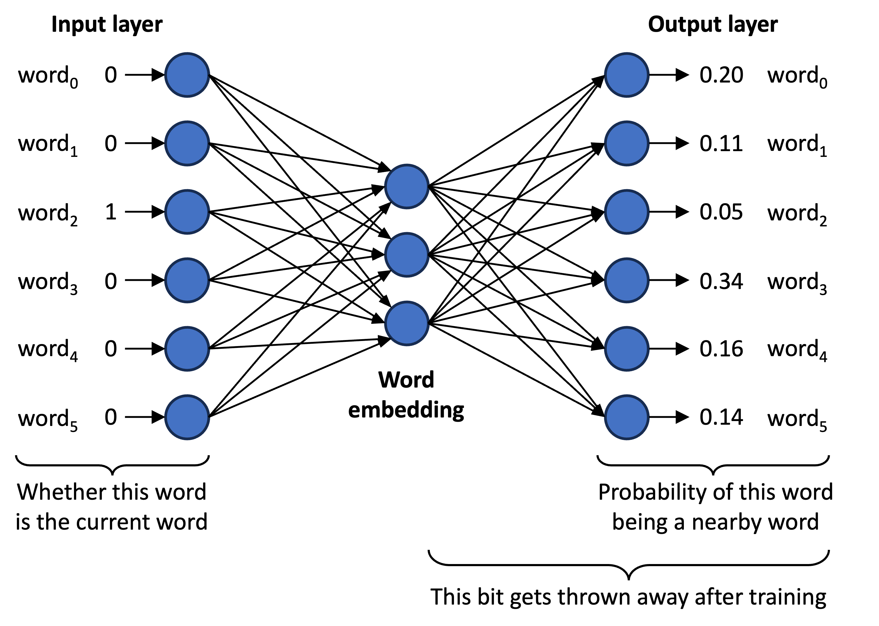
Like most forms of word embedding, word2vec learns an embedding using a large dataset of written text. Each word of each text sample is taken from this dataset in turn, and is input to the model using a one-hot encoding⁷. Unlike an autoencoder, the objective during training is not to generate the same values at the output layer as it receives at the input layer. Rather, it is to generate a probability distribution that captures the likelihood of each other word occurring in the surrounding text — though note that this is not what the trained embedding will actually be used for, and in practice the decoder tends to get thrown away after training.

During training, this probability distribution can be measured by looking at the actual surrounding text in the current sample, and so a loss function can be formulated that encourages the model to generate this distribution. Doing this over a large number of words in different text samples means that the decoder will eventually learn to generate appropriate distributions over its entire vocabulary. But more importantly, since similar words will tend to occur within similar distributions of surrounding words, these words will end up producing similar activations within the bottleneck layer. And consequently we can expect it to learn an embedding space that in some sense captures the relationships between words in its vocabulary.

In practice, the word embeddings produced by word2vec and other methods tend to be rather opaque, and do not necessarily capture relationships in a way that would be understandable to a human⁸. Nevertheless, they enabled a step-change in the ability of machine learning models to process text, and have become a key component within modern approaches to natural language processing — such as transformers.

Transformers

I’ll be covering transformers in a future post, so I won’t say a lot about them here. However, transformers are relevant to embedding spaces in two different ways. First, they use pre-trained word embeddings, such as word2vec⁹, to encode each word of their input text. Second, they create an embedding of all the text they receive as input.

This second use is most apparent within the original transformer architecture, which was designed for machine translation (i.e. translating text from one language to another), and consisted of an explicit encoder and an explicit decoder. The encoder was used to create a compressed embedding of the input text, and the decoder was then used to generate equivalent text in a different language. So, the embedding — which appeared as a pattern of activations within something analogous to a bottleneck layer — essentially captured the essence of the input text, but within a language-agnostic form which could then be decoded to different languages.

Modern transformer architectures are often described as being either encoder or decoder-based models. That is, they are said to consist of only an encoder or only a decoder, but not both. However, I find this terminology rather misleading, and the goal of the training process for both types of transformer is still essentially to produce an embedding. Take the GPT transformer architecture as an example. This is often referred to as a decoder model, since its goal is to generate text output. Yet, it also receives text as input, and prior to its final layer, embeds this text within a numeric feature vector. The final layer then does something akin to word2vec’s decoder, and turns this embedding into a probability distribution of next words.

Too long; didn’t read

Embeddings, aka latent spaces, are used to transform data into a compressed form that captures key information about the data. A common way of generating these embeddings is to use a bottleneck architecture, where a narrow layer within a neural network forces a compressed representation of the input data to be learnt. Embedding models are often trained in a way that encourages this representation to be meaningful in some way. Embeddings are commonly used in generative AI models, including transformers. They’re also used for feature reduction, anomaly detection and are generally useful for turning text into numbers.

1. Though of course there is a trade-off between the amount of compression and the amount of information loss; making the bottleneck too narrow means that it won’t be able to reconstruct the inputs at the outputs, likely making the model less useful.

2. For example, the reconstruction loss — which is calculated from the decoder’s output — can be useful in anomaly detection, since inputs that are less representative of a particular data distribution are more likely to be ignored during training and therefore are less likely to be successfully reconstructed by the autoencoder.

3. In practice, you’d probably use a convolutional autoencoder for this, which has convolution layers before and after the hidden layer(s).

4. In neural network terms, regularising.

5. This is not the only use case. Another common use case is sentiment analysis, e.g. when we want to train a classifier to tell us whether a passage of text is being nice or nasty — though this too is increasingly being done by transformers like ChatGPT.

6. You could try and pick these positions so that related words have 1s in nearby positions, but that’s not going to be easy, since each word is related to many other words in many different ways.

7. That is, there’s a separate input for each word in the model’s vocabulary, and only the input corresponding to the input word will have a value of 1; the others will all be 0.

8. For a discussion of some of the properties of word embeddings, see this paper.

9. These days they generally don’t use word2vec. The more advanced transformer models tend to include the learning of word embeddings within their broader training process, so they no longer use a separate word embedding model.