

I initially struggled to get my head around transformers. In an ideal world, it would be possible to read the paper that introduced them, Attention is All You Need, and absorb the relevant facts. But in practice this is a densely-written paper which assumes a lot of knowledge1. So, I also trawled through the introductions on the web, but these mostly frustrated me. Many of them only present the low-level details of the model, which are admittedly not that complicated, but which by themselves are not very revealing. Others attempt to describe how transformers work, but often in a way that’s hand-wavy and light on facts.
At the heart of it, I think there are several reasons why transformers are confusing:
They have a lot of moving parts, and these interact in complex ways that no one really understands.
Some of the design decisions are rather arbitrary, and informed by experiment rather than design — that is: oh, this works rather well, let’s keep it, rather than: ah, yes, that’s the obvious way of doing it.
The self-attention process, which is at the core of how transformers work, is not particularly intuitive, and is widely misunderstood.
In this post, I’m going to try to introduce transformers in a way that captures the key details but doesn’t require an understanding of linear algebra. To keep things simple, I’m going to stick to the kind of transformers that we’ve grown to know and love: GPT models (such as ChatGPT) which are used to generate text. The basic idea behind these is that you provide it with some text — in what is referred to as a context window2 — and it predicts the next word. This word then gets added to the end of the text, and the augmented text gets passed through the transformer again3, resulting in another word being produced. And so on4. In most cases this series of words will be the answer to a question you asked5.
For those who want more detail, take a look at the footnotes. I also recommend Jay Alammar’s “The Illustrated Transformer” if you want more depth than I provide here, though this does require understanding of basic linear algebra. If you’re more comfortable thinking in code, I’d also recommend Sebastian Raschka’s article on coding the self-attention mechanism.
Overall architecture
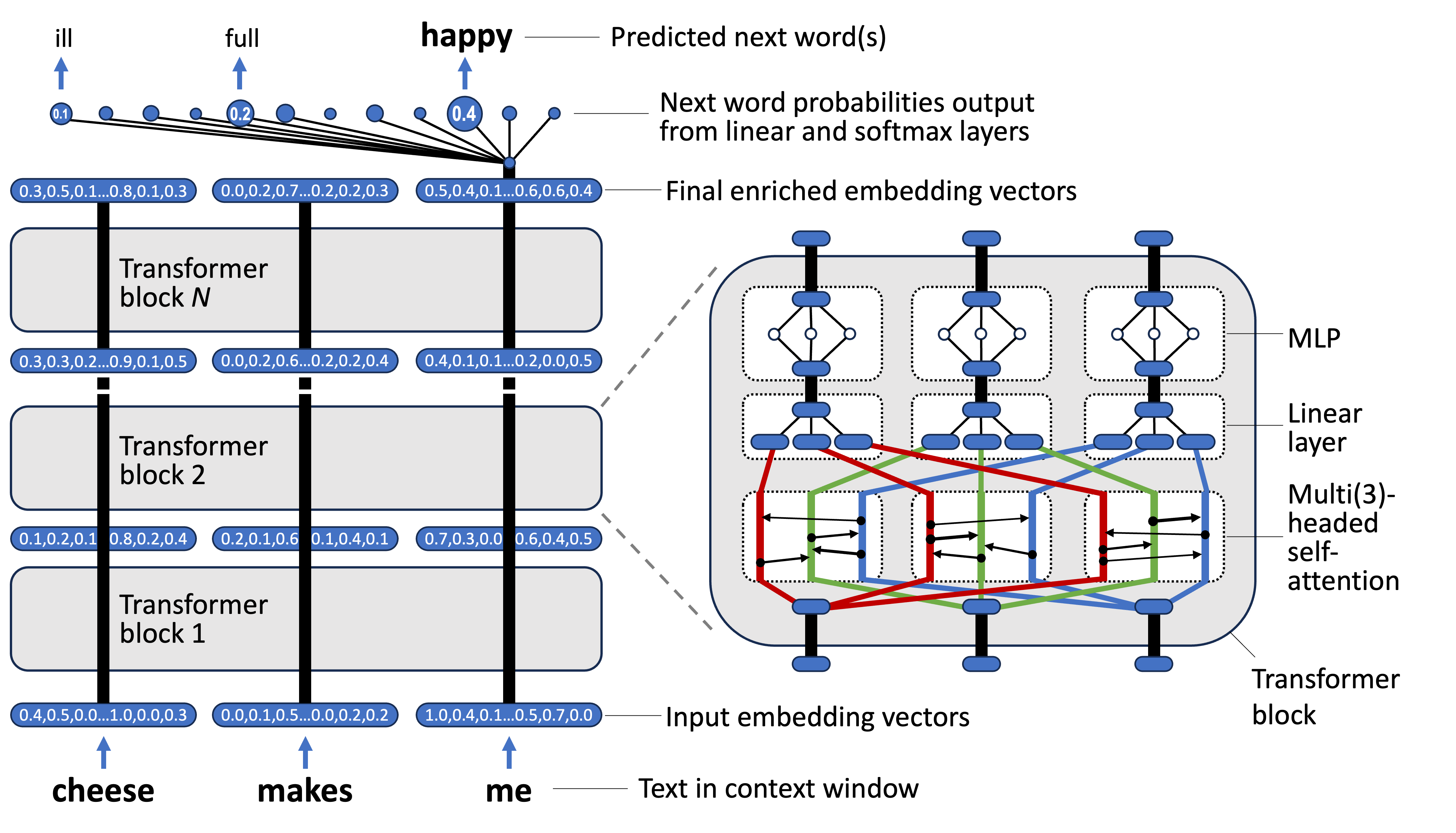
I think it helps to be aware of the overall architecture before looking at the details. These are some of the key points:
Transformers are organised into blocks. In each block is a self-attention layer followed by a multilayer perceptron (MLP for short, which I talked about in the first post in this series). Each block also contains some other, arguably less important, bits and pieces6.
The transformer block is repeated multiple times, with the outputs of each one feeding into the following one7. Each of these blocks has its own independent learnable weights, which are trained by a standard neural network optimiser in order to configure its behaviour (see Deep Dips #4: Training neural networks).
Importantly, the self-attention layer in each block is multi-headed. This means that the self-attention process (which I discuss below) is repeated multiple times, in parallel, with different weights, and then the outputs from each of these get combined before passing through the block’s MLP.
To give you some idea of scale, a self-attention layer in GPT-3 has 96 heads, and the whole thing comprises 96 transformer blocks. So that’s 96x96 = 9216 repeats of the self-attention process, each with different trainable weights. GPT-4, which underlies the most recent release of ChatGPT, presumably has a lot more8. This is worth bearing in mind before I get into the details of self-attention.
GPT is often referred to as a decoder-only model. However, this terminology only really makes sense within the context of the original transformer model, which was designed to translate one sequence of words into another. See my previous post on embedding models for more on this. It’s worth being aware that there are also encoder-only models like BERT, but in terms of how they work, encoder- and decoder-models are very similar. They only really differ in their output layers.
Input embedding
The way in which inputs to a transformer are represented is a key part of the puzzle of how they work, so I’m going to start here.
Neural networks process numbers, not text, so when a transformer receives text, each word9 must first be turned into a list of numbers — known as an embedding vector. A key idea underlying text-based transformers is that related words are represented by related embedding vectors. For example, if two words mean much the same thing, then they should have much the same embedding vector. If they have meanings that are different, but related, this is likely to be reflected in parts of their embedding vectors being similar and other bits being different.
The embedding process — turning words into embedding vectors — is not traditionally done by the transformer itself10. Rather, it’s done by a word embedding, which is many cases is another neural network. I talked about these in the previous post in this series, so I won’t repeat it here. Once the embedding process is complete, each of the input words will have been replaced by a corresponding embedding vector. In the case of GPT-3, for example, that turns out to be a vector (i.e. a list) of 12,288 numbers for each word. Multiplying that by the number of words in the context window means there’s a whole lot of numbers going into a transformer.
One thing to bear in mind is that because the word embedding used by a transformer is learnt from data, we don’t really know how it works. People have hypothesised that it might pick up on the same kind of relationships that humans recognise between words, but it’s quite possible that it has an entirely different outlook on things.
Oh, and there’s one more source of complexity in the input encoding, because transformers also impose a positional encoding on top of the embedding vectors. In the interest of not loading too much on you at once, I’ll come back to this later.
And let’s not forget the outputs
It sometimes helps to think of a transformer as a set of parallel pipelines (depicted as thick black lines in the diagram above), each one working at the same time on one word within the transformer’s context window. At the bottom of each pipeline enters an embedding vector representing the word. These embeddings then move up through each block of the transformer, and in each block they get transformed in some way. When they reach the top of the last transformer block, only the final embedding in the final pipeline (corresponding to the most recent word in the input context) gets used to predict the next word in the sequence.
I said earlier that GPT-style transformers generate a single word each time you use them. Well, that’s not entirely true. GPT-style transformers actually generate a probability distribution of next words, and this is then used to pick the next word. A temperature setting is often used to determine how this is done. A low temperature means that it will always pick the most likely next word, and a high temperature means it will often pick less likely words. That is, by twiddling the temperature knob on ChatGPT and friends you can vary the diversity of text generated.
So, how does the final embedding of the final word in the input text get turned into a probability distribution of next words? This is done using two more layers on top of the last transformer block. The first of these is a linear layer.
It’s worth pausing for a moment to explain what a linear layer is, since this concept will come up again later. A linear layer is essentially a fully-connected neural network layer that doesn’t use a transfer function. That is, every input is connected to every output, and the outputs are only determined by the layer’s weights11. This is different to a standard MLP layer, where the weighted sum of inputs is then fed through a non-linear transfer function. One common use of linear layers is to project data from one representation to another. And this is exactly what’s happening here. The linear layer contains an output node for each word in the transformer’s vocabulary12, and its inputs are the numbers in the final embedding of the final word, and it is essentially mapping between these two representations.
After the linear layer is a softmax layer, which is just a standard way of turning raw output numbers from a neural network into a probability distribution13.
Self-attention

At last we’ve reached the headline act of the transformer architecture, the self-attention layer. But things can get confusing at this point, and I find it helps to (a) not fixate on the term self-attention, which is far from being self-explanatory and (b) only think about the self-attention layer in the first transformer block. We can worry about the higher-ups later on.
The first self-attention layer receives as input a set of embedding vectors, one for each word in the context window. It then attempts to quantify how relevant each word is to every other word. Essentially, for each pair of embedding vectors (recall that each of these is a list of numbers), it does this by multiplying each pair of numbers within them together and then summing these values up14. This may sound a bit weird, but recall the idea from earlier that related words have related embeddings. This means that their embeddings are likely to contain, in places at least, big numbers at the same positions. So, if you multiply these numbers together, you’ll get even bigger numbers in the positions where they have commonalities, and the presence of these big numbers can be taken as an indication that these words are in some sense compatible with each other. So you can think of multiplying embedding vectors together as a general mechanism for amplifying their commonalities and thereby emphasising their relationships. Summing up all these multiplied-together numbers then produces a single number that captures how relevant two embeddings are to one another.
But it’s not quite that simple, because before they’re multiplied together, the embedding vectors are first altered by a bunch of learned weights, the purpose of which is to focus the search for relationships on particular parts of the embeddings. I use the word altered here to simplify things, but what actually happens is that each word embedding vector is multiplied by a weight matrix. However, this is not multiplication in the conventional arithmetic sense, but rather in a more specific linear algebra sense. But since I promised to avoid linear algebra, you can equivalently think of this as applying a linear layer (see above) to the embedding, in which the linear layer’s inputs are the numeric components of the word embedding, its outputs15 are the numeric components of the altered word embedding, and the weights in the linear layer correspond to the weights in the matrix.
And to further complicate matters, there are actually two separate weight matrices involved in this process, known as the key and query weight matrices. For each parallel pipeline, the key is applied to the pipeline’s own embedding vector and the query is applied to each of the others that it is being compared against — see the diagram above for a visual depiction of this. However, I wouldn’t worry too much about the distinction, since it’s really one of those oh, this works rather well, let’s keep it things I mentioned earlier, rather than being really integral to understanding what’s going on.
So, there are lots of learned weights involved in the self-attention process. To put the need for these in context, recall that each attention layer has multiple heads, i.e. multiple versions that are executed in parallel on the same set of embedding vectors. Since each of these has different learned weights, this means that each head can use its particular weight matrices to hone in on different parts of the embeddings, which in turn may correspond to particular aspects of language. So, one head might focus on what verbs are doing, another might be more concerned with adjectives, and others might be looking at more exotic relationships between words. Exotic here is code for “we have no clue what they might be doing.”
Essentially, the process described so far tells the self-attention layer how relevant each embedding vector is to each of the other embedding vectors in the context window. Now, recall earlier I mentioned that embedding vectors move up the transformer architecture in parallel pipelines. Well, the only place that information actually gets transferred between these pipelines is within the self-attention layers. And this is what happens next. For each pipeline, a new embedding vector is created by melding the existing embedding vector at that position with information taken from the other embedding vectors that the above process says are most relevant to it.
Specifically, this melding is done by creating a weighted sum of all the embedding vectors, with the weight assigned to each one determined by the strength of its relationship — as determined by the pairwise weight-multiply-and-sum process plus a bit of normalisation16. So, if embedding vector A has a strong relationship with embedding vector B, then quite a lot of A is going to end up in B, and vice versa. More generally, all the embedding vectors will gain information from the other embedding vectors that are most relevant to them.
But again it’s not quite that simple, because before the embedding vectors are weighted and summed, they each get multiplied by another learned weight matrix, known as the value weight matrix. Just like the key and query weight matrices earlier, this can be used to emphasise or de-emphasise certain parts of the embedding vectors during this integration process. And since different heads have different value weight matrices, this gives them yet another opportunity to specialise in particular aspects of language.
But don’t forget not self-attention
Despite its tendency to hog the limelight, there’s more to a transformer block than just self-attention. Two other important bits are the linear layer and the MLP layers.
The linear layer (yes, another one) is responsible for turning the embedding vectors generated by multiple heads back into a single embedding vector. That is, after the self-attention layer, at each word position, each self-attention head will have constructed a new embedding vector. So, a single original embedding vector will have become many, and to stop things getting out of hand, these need to become one again. It works just like the linear layers we came across earlier by taking the multiple embedding vectors (concatenated into one list of numbers) generated by each of the heads and mapping these to output values equal in number to the size of a single embedding vector, again configured using learnable weights.
This unified embedding vector then goes through the transformer block’s MLP. No one is entirely sure what the MLP does — again it depends on learned weights17 — but it’s basically the only opportunity for a transformer block to do something non-linear, since all the other operations described so far have been linear, and therefore limited in their ability to do interesting things. Despite the focus on self-attention within transformers, the majority of its parameters are actually in these MLP layers, so they’re an important, if not very well understood, part of the puzzle. And it’s worth noting that at this stage the embedding vectors are very much back in their parallel pipelines, and the same MLP is applied independently to each of them. So whatever it’s doing, it does it to each unified embedding vector separately, resulting in a bunch of altered embedding vectors that then become the inputs to the next transformer block.
Moving on up
So that’s how a transformer block is formulated: first carry out multi-headed self-attention, where information moves between related embedding vectors in different ways in each head, then apply a linear layer where the outputs of all the heads get munged together, and then do MLP, where something non-linear happens.
The first transformer block transforms the set of word embedding vectors in the context window into a new set of embedding vectors. This new set of embeddings are said to be enriched; that is, they’ve gained information by going through the self-attention and MLP process. People who know about these things reckon that the first transformer block tends to capture information about each word’s contextual relationship with nearby words — known as the local context.
These enriched embedding vectors then become the inputs to the second transformer block. Since these inputs already contain information about the local context, it is thought that the second block captures wider contextual relationships within the text, adding more nuance to the understanding of each word. Subsequent blocks then build upon this, further refining contextual understanding and finding broader meaning within the text in the context window.
However, much of this is speculation based upon observing particular trained transformers processing particular text samples, and in practice it’s very hard to know how transformers actually work, given their size and considerable complexity.
But what about position?
Oh yes, I promised to say something about positional encodings.
Something to be aware of is that transformers are by default ignorant when it comes to the position of words within the context window. This is because the self-attention process has no direct way of taking position into account — it just looks at every pair of embedding vectors, and treats them all equally. And this is a problem, because even us mere humans know that the position of a word within a sentence is a very important indicator of its role and meaning.
Positional encodings are a solution to this problem. They basically involve overlaying a positional encoding on top of each word’s embedding vector. That is, adding some numeric pattern to each embedding vector to give some indication of its position within the text. There are various ways of doing this, but one common way is to add some kind of repeating sinusoidal pattern to capture relative positions.
In theory, this means that the transformer has access to information about the positions of each pair of words when it is performing self-attention, and it can therefore take this context into account when enriching embedding vectors. In practice, it’s unclear (well, to me at least!) how the transformer then acts upon this information and integrates it with all the other information it’s processing. But I guess this is true of transformers in general.
And train
So that’s the main bits and pieces that make up a transformer. The final piece of the puzzle is how you configure it.
At this point it’s worth noting that the GPT in ChatGPT stands for Generative Pre-trained Transformer. That is, it isn’t just a transformer, but rather a transformer that has already been pre-trained by setting its learned weights to particular values. And it’s this particular configuration of weights that underlies its ability to generate meaningful text.
I’m not going to go into detail about how these weights are trained, since it basically involves using a standard neural network optimiser, which is something I plan to talk about in a future post. However, in a nutshell, these optimisers work by training on input-output examples, in which for a given input, the correct output is already known. The optimiser therefore knows what the output should be, and it can therefore determine how far the neural network missed it by. This information is then used to tweak the values of each weight, so that if the same input was provided again, it would get closer to the correct output. Doing this lots of times with lots of different input-output examples eventually leads to sensible weight values.
Exactly the same thing happens when training transformers. That is, they’re given some input, in the form of text. The correct output — the next word — is already known, so can be compared against whichever word the transformer predicts, and this error can then be used to tweak the weights. The only real difference is that transformers are a lot larger than other types of neural networks, and this basically means that a huge amount of input-output examples are required to train the weights correctly. For example, GPT-3 has 175 billion learnable weights and required about 500 billion words of text to train these weights18.
The end result is known as a large language model, or LLM. This is because, having absorbed a substantial fraction of all the text on the internet, the transformer has essentially learnt a generalised model of how humans use language. And it’s really this model, embedded in the weights of the transformer, that underlies the power of ChatGPT and its ilk.
Too long; didn’t read
Yes, it was quite long wasn’t it? I like to make these posts short, but transformers are just so darn complex. But I’ll attempt to make them simpler: A transformer consists of parallel pipelines within vertically-stacked blocks, with one pipeline working on each word in the transformer’s input text. Words are transformed into embedding vectors when they enter at the bottom, and in each block a combination of self-attention and multilayer perceptron layers enrich each embedding vector to capture contextual information and meaning from the other embedding vectors. The core operation of transformers, called self-attention, basically involves multiplying embedding vectors together in a pairwise fashion. This brings out their relationships, guided by a bunch of learned weights. A multilayer perceptron then increases the processing capacity of the block by adding non-linearity. Once it reaches the top of the transformer, the enriched embedding vector of the most recent word in the input should have gained all the context and meaning it needs to predict the next word in the text, and this is what happens. This predicted word gets added to the input, and the process repeats, generating subsequent words. It all works pretty well, but no one really knows how it works.
On top of this, the encoder-decoder transformer model described in this paper is mostly of historical interest.
Transformers can only look at so many words at once. The upper limit of this is known as the context window. For current transformers, this is typically in the 1000s of tokens, but some can handle much more than this.
Well, kind of. Most implementations have some way of maintaining internal state from previous iterations in order to improve efficiency.
This is known as autoregressive behaviour. It comes to an end when the transformer produces a special symbol called the end of sequence token.
Transformers like ChatGPT actually undergo two phases of training. In the first, and most important, phase, they’re trained to produce the next word in a sequence of text. In the second, they’re taught to interact in a question-and-answer style.
Including normalisation layers, which help to handle issues with gradients exploding during training.
There are also residual (or skip) connections between transformer blocks. This means a block can potentially feed into any other block higher up in the structure.
Its developer OpenAI is more like ClosedAI when it comes to releasing details.
Though generally this is done with tokens rather than words, since some words will be split into multiple tokens. For example, the word “working” might be split into “work” and “ing”.
Although some recent transformers train the embedding model and the transformer weights at the same time.
And, at least for the output layer, biases.
Typically in the order of tens of thousands.
Actually a pseudo-probability distribution. They’re not quite as mathematically well-behaved as real probability distributions, but they seem to work well in practice.
In linear algebra, this is known as the dot product between two vectors.
Typically the number of outputs is less than the number of inputs, so the altered embedding tends to be shorter than the original one. This is generally done for reasons of efficiency, so I wouldn’t worry too much about it. However, it helps to explain why the matrix multiplication operation in self-attention is sometimes described as projecting a word embedding into a representation subspace.
Actually two bits of normalisation, the first to control gradients, and the second to apply a softmax function so that the weights all sum to one. The details aren’t overly important.
Note that the weights of the linear layer and the MLP layers are both learned separately for each block of the transformer.
I wish I had this easy explanation while doing my Dissertation on Accountability in Private Large Language Models, but nevertheless this helps to clear some more basics. Great work!!